curve
Plots a one-dimensional curve in ℝ² or ℝ³.
Syntax
-
curve(data)-
datais a sequence of (X, Y) points
-
-
curve(data)-
datais a sequence of (X, Y, Z) points
-
-
curve(data)-
datais a sequence of (X, Y, Z, colour) points
-
Description
2D points
If data is a sequence of (X, Y) points, then curve(data) plots the curve obtained by connecting these points with straight lines.
Technically, data can be a plain sequence of points as function arguments, a list of points, or an n×2 real matrix in which each row represents a single point.
The curve is shown in the current diagram and a reference to the curve is returned.
The AdjustVisual function can be used to adjust the appearance of the curve. See Visual settings for a list of applicable settings.
3D points
Similarly, if data is a sequence of (X, Y, Z) points, then curve(data) plots the curve obtained by connecting these points with straight lines.
Technically, data can be a plain sequence of points as function arguments, a list of points, or an n×3 real matrix in which each row represents a single point.
The curve is shown in the current scene and a reference to the curve is returned.
The AdjustVisual function can be used to adjust the appearance of the curve. See Visual settings for a list of applicable settings.
Additionally, you can plot a curve in which each vertex has its own colour. To do this, let data be a sequence of (X, Y, Z, colour) points.
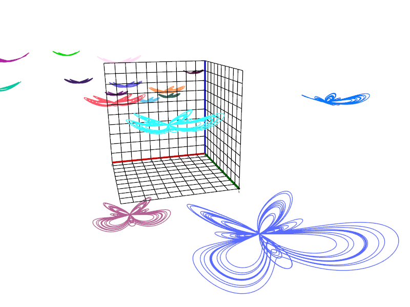
Examples
curve([0, 32⋅π] @ (t ↦ t⋅❨cos(t), sin(t)❩))

f ≔ t ↦ (e^sin(t) − 2⋅cos(4⋅t) + sin((2⋅t − π)/24)^5) ⋅ ❨cos(t), sin(t)❩;
B ≔ curve([0, 100, 0.01] @ f);
AdjustVisual(B, "line color": "salmon", "line width": 3)

f ≔ t ↦ (e^sin(t) − 2⋅cos(4⋅t) + sin((2⋅t − π)/24)^5) ⋅ ❨cos(t), sin(t)❩;
g ≔ (u, v) ↦ ❨u, v, u^2 / 10❩;
scene("butterflies");
L ≔ compute(❨RandomReal(−25, 25), RandomReal(−100, 40), RandomReal(−10, 10),
             integer(RandomColor())❩, k, 1, 20);
ForEach(L, v, curve([0, 100, 0.01] @ (t ↦ g(f(t))) @ ((x, y, z) ↦ ❨x, y, z, 0❩ + v)));
scene("butterflies")