plot

The generalised visualisation function.

Syntax

• plot(equation[, a, b[, δ]])

  • equation is an equation

• plot(inequality[, a, b[, δ]])

  • inequality is an inequality

• plot(inequalities[, a, b[, δ]])

  • inequalities is a chain of two inequalities

• plot(equation[, ❨xmin, xmax[, δx]❩, ❨ymin, ymax[, δy]❩[, opts]])

  • equation is an implicit equation

  • xmin, xmax, and δx are real numbers

  • ymin, ymax, and δy are real numbers

  • opts is a string containing zero or more of i and s

‣ Note: Vector brackets can be inserted by pressing Shift+Ctrl+V.

• plot(data)

  • data is a sequence of (X, Y) points

• plot(data)

  • data is a sequence of (X, Y, Z) points

• plot(data)

  • data is a sequence of (X, Y, Z, colour, radius) points

Description

Explicit equations

If equation is an equation in the Cartesian coordinates x and y with either the LHS or the RHS equal to one of these variables and the other side not containing this variable, then plot(equation) plots this function curve.

Examples:

y = sin(x)
x = √y + 1
ln(x) + 4 = y

If inequality is an inequality in the Cartesian coordinates satisfying the same restrictions, then the implied planar region is plotted.

Examples:

y < sin(x)
x > √y + 1
ln(x) + 4 < y

If inequalities is a chain of two inequalities in the Cartesian coordinates x and y and at least one side is such a variable isolated and the remaining sides functions of this variable, then the implied region (the region between two function curves) is plotted.

Examples:

sin(x) < y < 2⋅sin(x)

In all these cases, the plot is taken as the independent variable goes from a to b in steps of δ; if omitted, a default value is used for each parameter.

Implicit equations

If equation is an implicit equation in the Cartesian coordinates x and y, then plot(equation) plots the implied planar region within the [−10, 10]² square. To specify an explicit rectangular region, speciy the xmin, xmax, ymin, and ymax parameters. The function will sample the scalar field

F(x, y) = LHS − RHS

equivalent to the specified equation LHS = RHS at the points of a regular grid within [xmin, xmax] × [ymin, ymax]. A default resolution is used in each dimension, so that the total number of samples is about 250 000; this default value can be changed in the Algosim settings (Numerics_ContourSamplesPerAxis).

An explicit resolution can be specified in each direction by giving the steps δx and δy as arguments.

The plot function determines the contour by means of a “marching squares” algorithm with interpolation. The contour produced is then investigated to see if it can be simplified. Chiefly, segments of straight lines are conics are detected. In the first case, the vertices in a straight-line segment are replaced by only the endpoints.

If omitted, the opts (options) parameter is set to "is", which means that the interpolation (i) and simplification (s) steps are to be performed. Each of these steps can be suppressed by explicitly specifying a different value of opts (such as "i", "s", or the empty string "").

Plotting raw data

plot(data) is the same as ScatterPlot(data).

The plot is shown in the current diagram (for 2D plots) or scene (for 3D plots) and a reference to the plot is returned.

Examples

plot(y = sin(x), −π, π)

plot(cos(x) < y < 2⋅cos(x), −π, π)

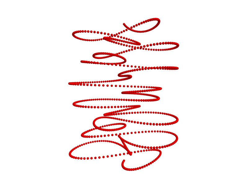
plot([−2⋅π, 2⋅π] @ (t ↦ ❨5⋅cos(5⋅t)⋅sin(5⋅t), 5⋅sin(5⋅t)⋅sin(2⋅t), t❩))

plot(sin(x)^4 + sin(y)^4 = 1, ❨−π, π❩, ❨−π, π❩)

Compare this contour with the following visualisation:

scene("trig");
surf(z = sin(x)^4 + sin(y)^4, ❨−π, π❩, ❨−π, π❩);
surf(z = 1, ❨−π, π❩, ❨−π, π❩)

See also

• ContourPlot

• graph

• ScatterPlot

• LinePlot

• AreaChart

• curve

• surf