ScatterPlot
Creates an XY or XYZ scatter plot.
Syntax
-
ScatterPlot(data)-
datais a sequence of (X, Y) points
-
-
ScatterPlot(data)-
datais a sequence of (X, Y, Z) points
-
-
ScatterPlot(data)-
datais a sequence of (X, Y, Z, colour, radius) points
-
Description
2D points
If data is a sequence of (X, Y) points, then ScatterPlot(data) creates a scatter plot from this data.
Technically, data can be a plain sequence of points as function arguments, a list of points, or an n×2 real matrix in which each row represents a single point.
The chart is shown in the current diagram and a reference to the chart is returned.
To plot the graph of a function using points only, you may combine ScatterPlot with the graph function. But it is more convenient to use plot instead.
3D points
Similarly, if data is a sequence of (X, Y, Z) points, then ScatterPlot(data) creates a scatter plot from this data.
Technically, data can be a plain sequence of points as function arguments, a list of points, or an n×3 real matrix in which each row represents a single point.
The chart is shown in the current scene and a reference to the chart is returned.
To plot the graph of a function using points only, you may combine ScatterPlot with the graph function. But it is more convenient to use plot instead.
Additionally, you can plot a set of points in which each point has its own colour and radius. This set needs to be a set of (X, Y, Z, colour, radius) points, and can be specified in any of the ways described above for (X, Y, Z) point sets.
Examples
2D points
ScatterPlot(❨1, 1❩, ❨2, 5❩, ❨3, −2❩)
or
ScatterPlot('(❨1, 1❩, ❨2, 5❩, ❨3, −2❩))

A ≔ ❨❨1, 1❩, ❨2, 5❩, ❨3, −2❩❩
⎛ 1   1⎞
⎜ 2   5⎟
⎝ 3  −2⎠
ScatterPlot(A)
ScatterPlot(graph(sin, −2⋅π, 2⋅π))

3D points
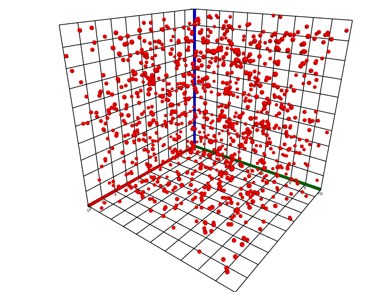
ScatterPlot(10⋅RandomMatrix(1000, 3))
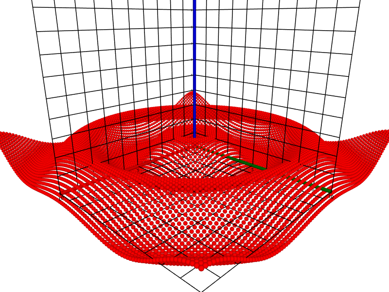
ScatterPlot(graph((x, y) ↦ sin(√(x^2 + y^2)), ❨−10, 10❩, ❨−10, 10❩))
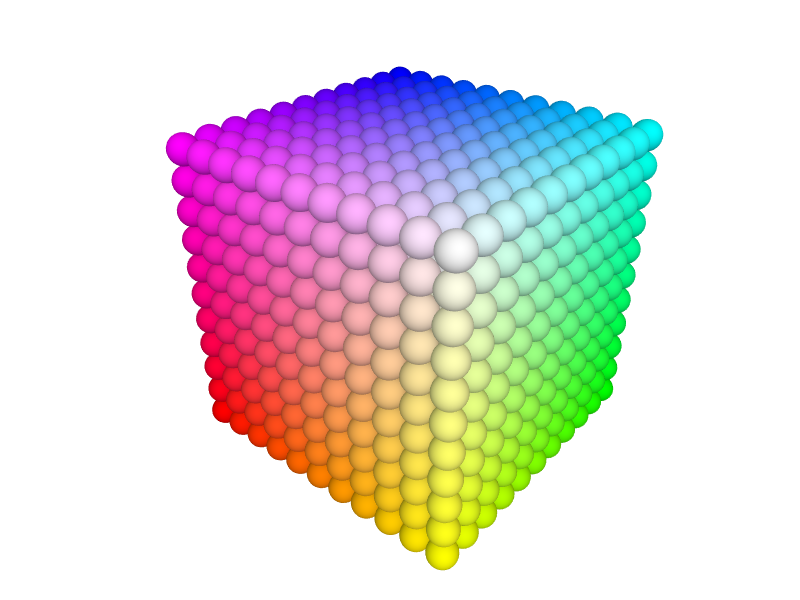
F ≔ (x, y, z) ↦ ❨x, y, z, integer(rgb(x / 10, y / 10, z / 10)), 5.0❩;
ScatterPlot([0, 10, 1]^3 @ F)
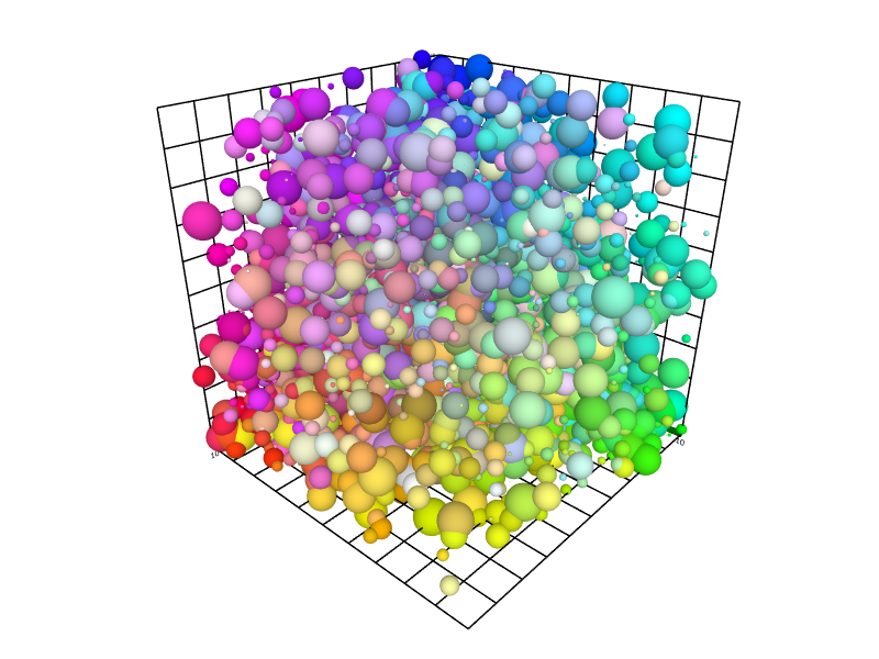
F ≔ (x, y, z) ↦ ❨x ⋅ RandomReal(), y ⋅ RandomReal(), z ⋅ RandomReal(), integer(rgb(x / 10, y / 10, z / 10)), RandomReal(5.0)❩;
ScatterPlot([0, 10, 0.5]^3 @ F)
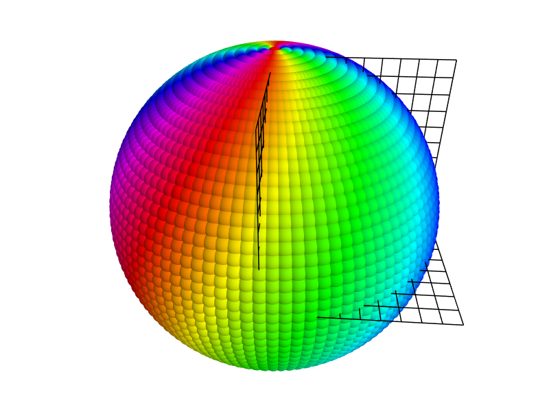
F ≔ (θ, φ) ↦ ❨10⋅sin(θ)⋅cos(φ), 10⋅sin(θ)⋅sin(φ), 10⋅cos(θ), integer(hsv(180⋅(θ+2⋅φ)/π, 1.0, 1.0)), 5.0❩;
ScatterPlot([0, π, π/50] × [0, 2⋅π, π/50] @ F)
What about 1D points?
The above discussion details how to plot a sequence of points in ℝ² or ℝ³. But what if you have a list (or vector) containing real numbers, that is, elements of ℝ? Like this:
3.1, 2.9, 3.5, 3.2, 3.4, 3.0, 2.9, 3.7, 3.2, 3.5
One way to visualise such a sequence is to transform it into a sequence of points in ℝ²:
(1, 3.1), (2, 2.9), (3, 3.5), (4, 3.2), (5, 3.4), (6, 3.0), (7, 2.9), (8, 3.7), (9, 3.2), (10, 3.5)
Then this sequence can be plotted as before. To accomplish this, one can use the SequenceVector function along with MatFromCols:
D ≔ ❨3.1, 2.9, 3.5, 3.2, 3.4, 3.0, 2.9, 3.7, 3.2, 3.5❩;
plot(MatFromCols(SequenceVector(#D), D))

See the example in LineSegment for a different approach, in which a one-dimensional diagram is used to visualise a monotonic sequence.