Visualization

Algosim contains quite a few visualization functions that are used to draw plots and diagrams, such as

scatter plots (points, lines, regions),
curves and surfaces,
bar charts,
histograms,
pie charts,
vector fields,
heatmaps, and
geometric objects.

Please see Visualization functions for detailed descriptions of all these functions.

This article, however, tries to give a conceptual overview of the facilities used to plot mathematical curves and surfaces of various kinds from a mathematical point of view, not a technical point of view.

Drawing a plane curve expressed as an equation in Cartesian coordinates

Given an equation f(x, y) = 0 in the Cartesian coordinates x and y, the set { (x, y) ∈ ℝ² : f(x, y) = 0 } can be drawn easily using the plot function. If the equation has one of the Cartesian coordinates isolated (alone) on one side, plotting is performed by (the natural) parameterisation, which is very efficient.

plot(y = sin(x))

plot(x = y^2 + 10⋅sin(y))

It’s also possible to plot regions defined similarly:

plot(cos(x) < y < 2⋅cos(x), −π, π)

Again, this is a very computationally efficient plot since the y coordinate is isolated.

However, the plot function can also produce implicit plots from any equation in the Cartesian coordinates:

plot(x^4 + x^3⋅y + y^4 = arctan(x + y))

In this case, a “marching squares” algorithm is used to produce a contour.

Drawing a graph of a function of a single real variable

Given a function f: D_f → ℝ, its graph is the set { (x, y) ∈ ℝ² : x ∈ D_f ∧ y = f(x) }.

Although the above method clearly can be used to draw graphs, it is also possible to use the graph function:

curve(graph(arctan, −10, 10))

Drawing a parameterised plane curve

Given a function F: D_F → ℝ² where D_F ⊂ ℝ, the image of an interval [a, b] ⊂ D_F under F is a curve and can be plotted directly using curve:

F ≔ t ↦ t⋅❨cos(t), sin(t)❩;
curve([0, 6⋅π] @ F)

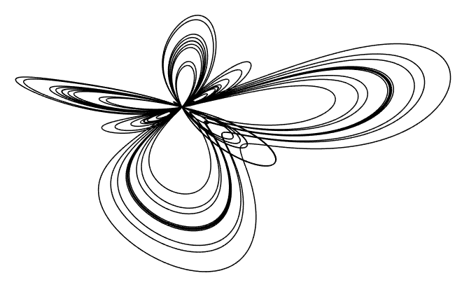
f ≔ t ↦ (e^sin(t) − 2⋅cos(4⋅t) + sin((2⋅t − π)/24)^5) ⋅ ❨cos(t), sin(t)❩;
curve([0, 100, 0.01] @ f)

Drawing a surface expressed as an equation in Cartesian coordinates

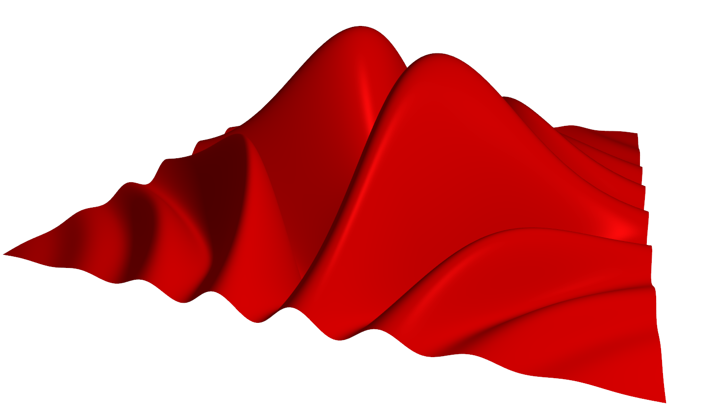
Given an equation f(x, y, z) = 0 in the Cartesian coordinates x, y, and z, the set { (x, y, z) ∈ ℝ³ : f(x, y, z) = 0 } can be drawn directly assuming the equation can be rewritten so that one of the variables is isolated on one side of the equation.

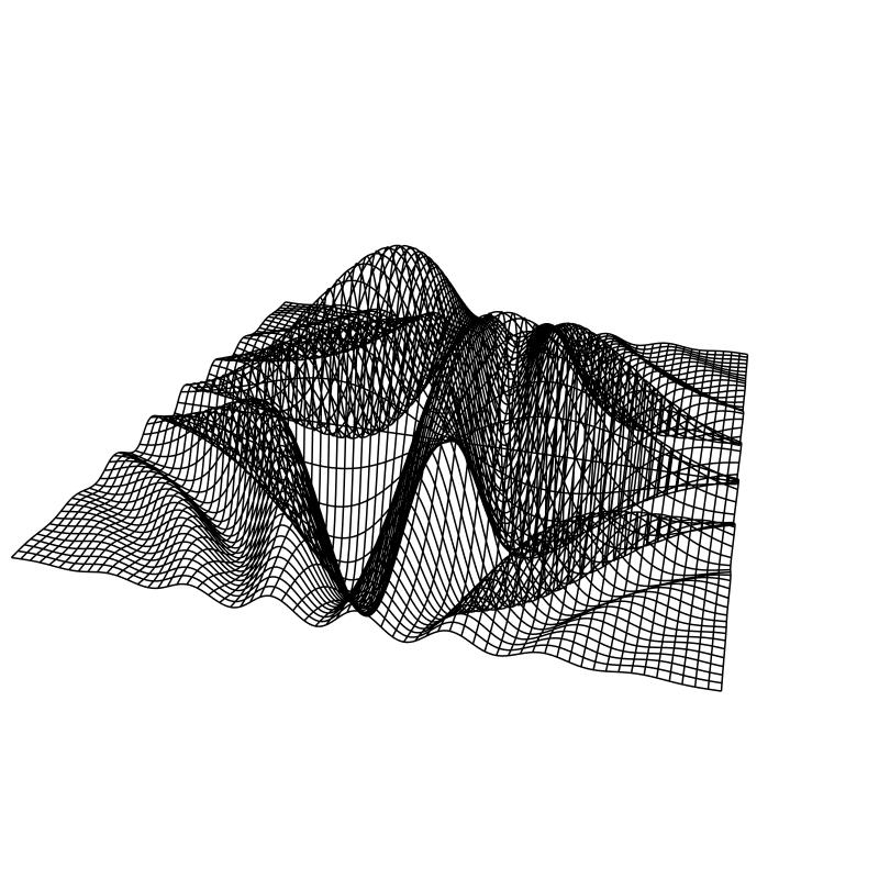
surf(z = 6⋅sin(x⋅y/4)⋅arctan(2⋅√(x^2+y^2))⋅exp(−(x^2+y^2)/32))

Or,

AdjustVisual(ans, "show surface": false, "show parameter curves": true)

Drawing a parameterised surface

Given a function F: D_F → ℝ³ where D_F ⊂ ℝ², the image of a rectangle [a, b]×[c, d] ⊂ D_F under F is a surface and can be plotted directly:

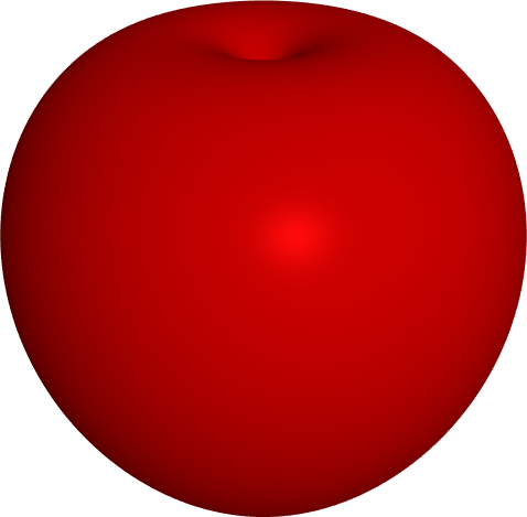
F ≔ (θ, φ) ↦ θ⋅❨sin(θ)⋅cos(φ), sin(θ)⋅sin(φ), cos(θ)❩;

surf([0, π] × [0, 2⋅π] @ F)

Drawing a parameterised space curve

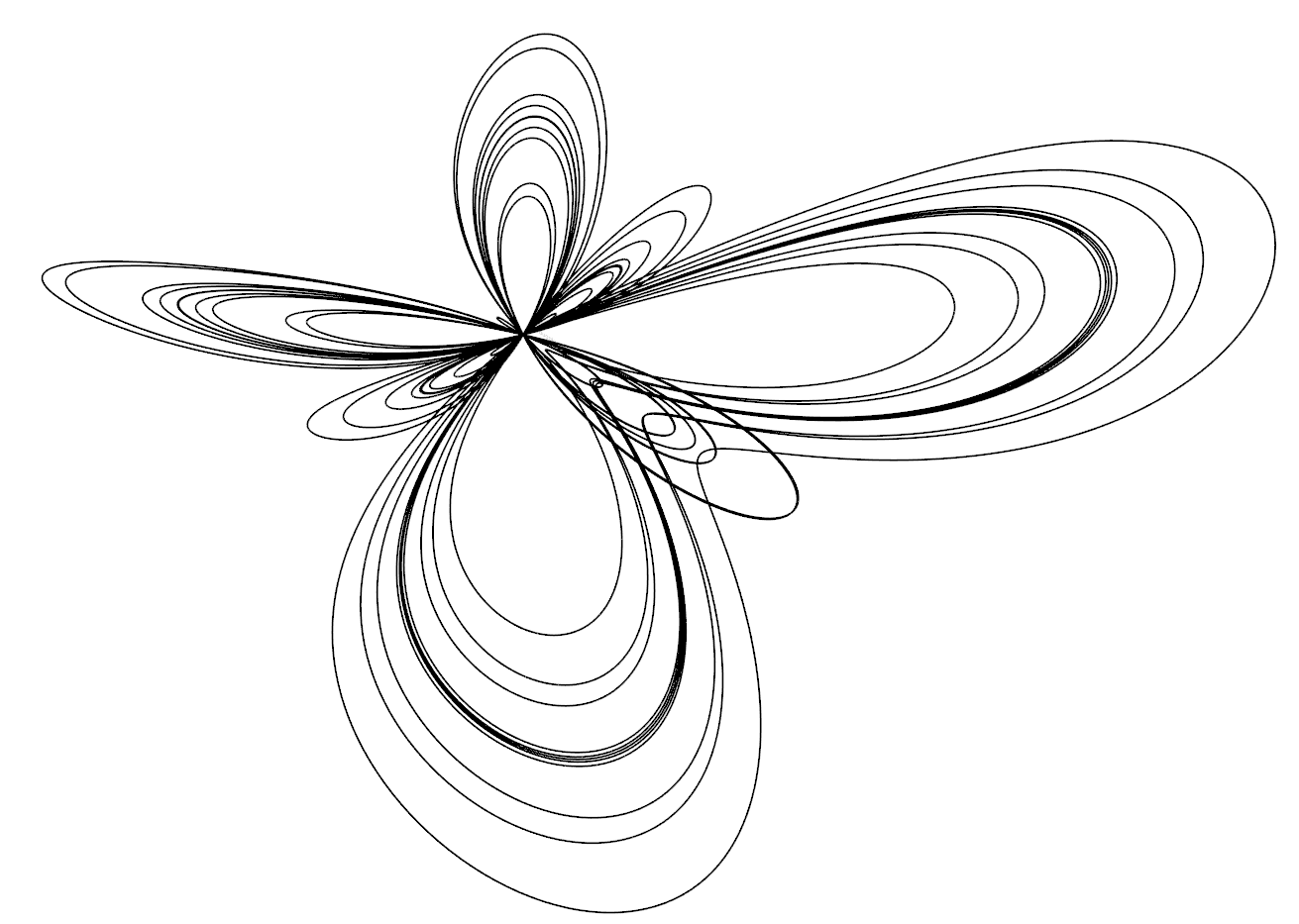
f ≔ t ↦ (e^sin(t) − 2⋅cos(4⋅t) + sin((2⋅t − π)/24)^5) ⋅ ❨cos(t), sin(t)❩;
g ≔ (u, v) ↦ ❨u, v, u^2 / 10❩;
curve([0, 100, 0.01] @ (t ↦ g(f(t))))

Visualizing two-dimensional scalar field

Plotting a surface z = f(x, y) is just one way of visualizing a two-dimensional scalar field f.

You can also plot its level sets (level curves, contours) or make a heatmap.

For example,

f ≔ (x, y) ↦ 6⋅sin(x⋅y/4)⋅arctan(2⋅√(x^2+y^2))⋅exp(−(x^2+y^2)/32);

surf(z = f(x, y))

ContourPlot(f, ❨−10, 10❩, ❨−10, 10❩)

heatmap(f, ❨−10, 10❩, ❨−10, 10❩)

diagram("scalar field");

heatmap(f, ❨−10, 10❩, ❨−10, 10❩);

ContourPlot(f, ❨−10, 10❩, ❨−10, 10❩)