VectorField

Creates a vector field plot in ℝ² or ℝ³.

Syntax

• VectorField(f, ❨xmin, xmax[, δx]❩, ❨ymin, ymax[, δy]❩)

  • f is a function D → ℝ² where D ⊂ ℝ²

  • xmin, xmax, ymin, and ymax are real numbers

  • δx and δy are non-negative real numbers

• VectorField(f, ❨xmin, xmax[, δx]❩, ❨ymin, ymax[, δy]❩, ❨zmin, zmax[, δz]❩)

  • f is a function D → ℝ³ where D ⊂ ℝ³

  • xmin, xmax, ymin, ymax, zmin, and zmax are real numbers

  • δx, δy, and δz are non-negative real numbers

• VectorField(f, ❨xmin, xmax[, δx]❩, ❨ymin, ymax[, δy]❩, ❨zmin, zmax[, δz]❩)

  • f is a function D → ℝ⁴ where D ⊂ ℝ³

  • xmin, xmax, ymin, ymax, zmin, and zmax are real numbers

  • δx, δy, and δz are non-negative real numbers

• VectorField(data)

  • data is a sequence of points in ℝ⁶ or ℝ⁷

Description

Planar vector fields

The VectorField function creates a plot of the vector field f in the rectangular region [xmin, xmax] × [ymin, ymax] with a sampling distance of δx in the first dimension and δy in the second dimension. The sampling distance is the distance between arrows. If omitted, a reasonable default value is used (typically producing a plot with about 20 arrows along each direction).

The plot is shown in the current diagram and a reference to the plot is returned.

Vector fields in space

The VectorField function creates a plot of the vector field f in the box [xmin, xmax] × [ymin, ymax] × [zmin, zmax] with a sampling distance of δx in the first dimension, δy in the second, and δz in the third. The sampling distance is the distance between arrows. If omitted, a reasonable default value is used (typically producing a plot with about 20 arrows along each direction).

In addition to an ordinary vector field D → ℝ³, the VectorField function can also be given a mapping D → ℝ⁴ where each image is of the form ❨x, y, z, colour❩, the fourth component being the integral representation of the arrow’s colour at ❨x, y, z❩.

The plot is shown in the current scene and a reference to the plot is returned.

Vector fields on parameterised manifolds

The above approach to plotting a vector field in space requires the domain to be a rectangular cuboid. The VectorField(data) approach relaxes this requirement; in particular, it lets the user plot a vector field along a curve or surface.

If data is a sequence of points in ℝ⁶ of the form ❨x, y, z, u, v, w❩, then VectorField(data) draws the vector field obtained by plotting ❨u, v, w❩ at ❨x, y, z❩. If data is a sequence of points in ℝ⁷ of the form ❨x, y, z, u, v, w, c❩, where c is an integral colour code, the vector at ❨x, y, z❩ will be drawn in the colour c.

data may be a sequence of vectors, a single list of vectors, or an n×6 (n×7) matrix in which each row represents a single vector field arrow.

Examples

D ≔ diagram("vector field");
sf ≔ heatmap((x, y) ↦ x^2 + y^2, ❨−10, 10❩, ❨−10, 10❩, '("white", "red"));
vf ≔ VectorField((x, y) ↦ ❨2⋅x, 2⋅y❩, ❨−10, 10❩, ❨−10, 10❩)

D ≔ diagram("field");
disk(❨0, 0❩, .3);
F ≔ (x, y) ↦ ❨−y, x❩ / (x^2 + y^2)^1.5;
vf ≔ VectorField(F, ❨−2, 2, .5❩, ❨−2, 2, .5❩);
AdjustVisual(vf, "arrow-scale": 4, "auto-normalize": true);

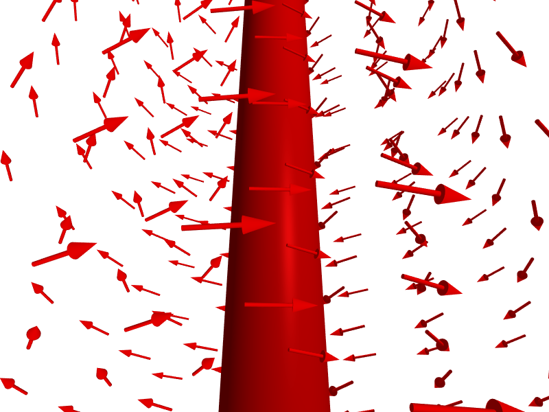
scene("field");
C ≔ cylinder(❨0, 0, −10❩, ❨1, 1, 20❩);
F ≔ (x, y, z) ↦ ❨−y, x, 0❩ / (x^2 + y^2)^.5;
VF ≔ VectorField(F, ❨−5, 5, 2❩, ❨−5, 5, 2❩, ❨−10, 10, 2❩)

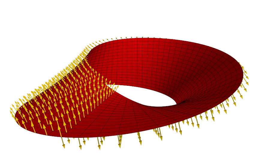
NF ≔ F ↦ ((u, v) ↦ normalized(diff(F(u, v), u, u) × diff(F(u, v), v, v)));

S ≔ ClearScene("Möbius strip");
AdjustVisual(S.axes, "visible": false);
AdjustVisual(S.view, "rθφ": ❨2.792, 72°, 20°❩);

F ≔ (u, v) ↦ ❨(1 + .5⋅v⋅cos(u/2))⋅cos(u), (1 + .5⋅v⋅cos(u/2))⋅sin(u), .5⋅v⋅sin(u/2)❩;
M ≔ surf([0, 2⋅π] × [−1, 1] @ F);
AdjustVisual(M,
  "show parameter curves": true,
  "parameter curve counts": ❨64, 16❩,
  "line width": .75,
  "unisided": true);

N ≔ NF(F);
VF ≔ VectorField([0, 2⋅π, π/32] × [−1, 1, 1/8] @ ((u, v) ↦ F(u, v) ~ N(u, v)));
AdjustVisual(VF,
  "size": 0.1,
  "anchor point": 1.03,
  "color": "gold")

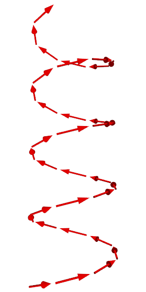
VF ≔ VectorField([−4⋅π, 4⋅π, π/4] @ (t ↦ ❨cos(t), sin(t), t/4, −sin(t), cos(t), 1/4❩));
AdjustVisual(VF, "size": .75)

See also

• heatmap